── Attaching core tidyverse packages ──────────────────────── tidyverse 2.0.0 ──
✔ dplyr     1.1.4     ✔ readr     2.1.5
✔ forcats   1.0.0     ✔ stringr   1.5.1
✔ ggplot2   3.5.2     ✔ tibble    3.2.1
✔ lubridate 1.9.4     ✔ tidyr     1.3.1
✔ purrr     1.0.4
── Conflicts ────────────────────────────────────────── tidyverse_conflicts() ──
✖ dplyr::filter() masks stats::filter()
✖ dplyr::lag()    masks stats::lag()
ℹ Use the conflicted package (<http://conflicted.r-lib.org/>) to force all conflicts to become errors
library(car)
Loading required package: carData

Attaching package: 'car'

The following object is masked from 'package:dplyr':

    recode

The following object is masked from 'package:purrr':

    some
Analysis of Covariance
The ANOVA allows us to analyze the effect of various levels of an independent variable on the dependent variable. The t test is used for two groups that vary based on the presence of an independent variable, but the ANOVA allows us to look at 3 or more groups. The ANCOVA is used when analyzing levels of an independent variable adjusted based on the expected effect of another second variable (Field).
In this case, the second variable is typically a continuous variable and usually functions as a type of pre-existing condition. So the second variable is not something manipulated in the experiment, but still thought to effect the relationship between the independent and dependent variable. This second variable is called a covariate.
ANOVA Review
Remember that the ANOVA or F statistic is based on comparing the explained variance or variance we can attribute to the manipulation of the independent variable to the unexplained variance or variance attributed to measurement error. So the basic comparison is between the variation between the groups compared to the variation within the groups.
\[
\frac{SS_{between}}{SS_{within}}
\] However it takes a few more steps to get to the F value base on the mean squares \(MS\), so the full formula looks like this: \[
\frac{SS_{between}/df_{between}}{SS_{within}/df_{within}} = \frac{MS_{between}}{MS_{within}}= F
\]
ANOVA in R Studio
When performing ANOVA in R Studio, we use the general linear model, which is highly related to ANOVA, so the basic formula in R Studio looks like this with \(M\) standing for Model and \(R\) standing for residuals:
\[
\frac{SS_{M}}{SS_{R}}
\]
Confounds
One of the primary issues in experimental design is confounds. Confounds are other variables (sometimes called nuisance variables) besides the independent variable that have an effect on the dependent variable. So a lot of work in experimental design is trying to control for or eliminate confounds, which is why experimental psychologists work so hard to try and have everything the same in the control and experimental conditions, except for the manipulation of the independent variable.
Reducing Error Variance
The ANCOVA tries to account for other potential confounds by reducing the within groups error variance \(SS_R\). \(SS_R\) is variance that is unexplained. So if part of that unexplained variance can be accounted for by another variable (the covariate) it increases the likelihood of detecting a real effect of the independent variable.
The covariate is typically a variable that effects the relationship between the independent variable and the dependent variable, but is not likely to be something that could be manipulated in an experiment. This is often because it is something that is a pre-existing condition or a variable that develops in individuals participants over time.
Revisiting Some Mischief
For the section on the independent t test, we looked at the effect of an invisibility cloak on acts of mischief. The idea was that if you had an invisibility cloak (like the one used by Harry Potter to explore Hogwarts) you might be more inclined to do more types of mischief.
However, a potential covariate would be how mischievous you are more generally. So if you are already someone who is always getting into trouble (pulling pranks, being sent to the principal’s office, often serving detention, etc), you are already more likely to do a lot of mischief before you get access to an invisibility cloak. So an ANCOVA allows for a participant’s previous mischief to be accounted for when exploring the relationship between the primary relationship between the invisibility cloak and mischief. This would help to separate the influence of being mischievous more generally from the effect of the invisibility cloak on mischievous behavior.
In this case, mischief1 is the baseline level of mischief or how often a subject engages in mischievous acts on a regular basis. Baseline data is used in a lot of different situations to refer to how persons perform on a variable in everyday situations. So you might think about a baseline heart rate or a baseline level of religiosity. So prior to any experimental manipulation, baseline gives you the current level of some measure of a variable.
An Example with Puppies
Let’s look at an example using puppies or more specifically using puppies as a form of therapy (Field). Here’s the dataset.
The independent variable is Dose. There are three levels to the independent variable (Control, 15 mins, and 30 mins), which refers to the amount of time spent with the puppies.
Puppy_love$Dose
<labelled<double>[30]>: Dose of puppies
 [1] 1 1 1 1 1 1 1 1 1 2 2 2 2 2 2 2 2 3 3 3 3 3 3 3 3 3 3 3 3 3

Labels:
 value   label
     1 Control
     2 15 mins
     3 30 mins
The dependent variable would be Happiness, which refers to the amount of happiness participants experienced after spending time with the puppies, which is on a 0-10 point scale.
Alternative - Puppy therapy has an effect on happiness
As before, the first step will be to turn Dose into a factor to better show the levels of the independent variable. This time we’ll use the tidyverse to modify this type of variable
# A tibble: 3 × 3
Dose n mean
<fct> <int> <dbl>
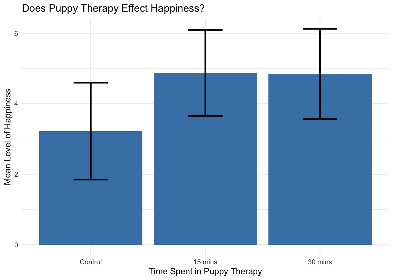
1 Control 9 3.22
2 15 mins 8 4.88
3 30 mins 13 4.85
Notice that there is no real difference between 15 mins and 30 mins of puppy therapy, but there is a difference between the control group and both 15 and 30 mins of puppy therapy. Next, we’ll need to run the ANOVA to decide if this mean difference is significant or not.
Puppy Love ANOVA
To run the ANOVA we need to use the aov argument and save it as an object.
Puppy_ANOVA <-aov(Happiness ~ Dose, data = Puppy_love)
Once the ANOVA has been saved, we can look at the results
summary(Puppy_ANOVA)
            Df Sum Sq Mean Sq F value Pr(>F)
Dose         2  16.84   8.422   2.416  0.108
Residuals   27  94.12   3.486
Notice that the F value is not significant. It’s only 2.416 with a p value of 0.1008. So on the face of it, it would appear that Puppy therapy doesn’t have an effect on happiness. This is where looking at the influence of a covariate might be helpful. The ability for puppy therapy to have an effect on your level of happiness would certainly be related to whether or not you liked puppies in the first place! Perhaps you are not a dog lover or you’ve had negative experiences with dogs. If we can account for the influence of this covariate, it may help us to see if puppy therapy actually has an effect on happiness.
In the dataset, the covariate is lised as Puppy_love and is based on a 0 to 7 scale.
The code for this model is changed slightly to account for the covariate, Puppy_love.
Puppy_ANCOVA <-aov(Happiness ~ Dose + Puppy_love, data = Puppy_love)
To look at the results we have to use a slightly different version of ANOVA (“type = III”) using the car package. So this is what the summary looks like
The first thing to notice here is that the variable Dose is now significant with an F value of 4.1419 and a p value of 0.02745. Puppy_love is also significant with an F value of 4.9587 and a p value of 0.03483.
If you look back at the original ANOVA, the residual sum of squares is 94.12. Notice that here the residual sum of squares is 79.047, so the inclusion of the co-variate has reduced the residual sum of squares. It’s important to note that the total sum of squares or total variance has not changed, but how that variance has been accounted for has changed, which changes the overall results.
Effect size for ANCOVA
The effect size for ANCOVA uses something slightly different then the eta squared \(\eta^2\) we used for the ANOVA called a partial eta squared. It is a proportion of variance that a variable explains in comparison to the variance not explained by other variables. Here is the formula.
So you look at the sum of squares for the effect of interest (in this case, either the independent variable or covariate) then divide by that same effect plus the residual. Here is the formula for the independent variable Dose.
\[
Dose=\frac{25.185}{25.185+79.047}
\]
In R Studio
25.185/(25.185+79.047)
[1] 0.2416245
And then the formula for the covariate Puppy_love
\[
Puppy_love=\frac{15.076}{15.076+79.047}
\]
In R Studio
15.076/(15.076+79.047)
[1] 0.1601734
So writing out the results looks like this:
The covariate, love of puppies, was significantly related to the participant’s happiness, F(1, 26) = 4.96, p = 0.035, partial \(\eta^2\) =0.16. There was also a significant effect of puppy therapy on levels of happiness after controlling for the effect of love of puppies, F(2, 26) = 4.14, p = 0.027, partial \(\eta^2\) = 0.24.
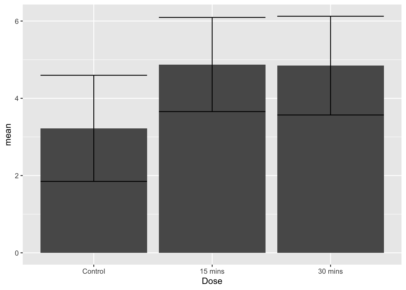
Graphing the results
For graphing the results, a bar graph is the best way to look at the means. We can use the same basic formula we used for the one way anova to find our descriptive statistics.