sprint <- c(18, 16, 18, 24, 23, 22, 22, 23, 26, 29, 32, 34, 34, 36, 36, 43, 42, 49, 46, 46, 57)Hypothesis Testing
Populations and Samples
So far, we’ve primarily dealt with descriptive statistics, which are used to describe the basics of a dataset (think central tendency and variability). However, most of psychological science is running experiments and testing hypotheses. When psychologists run an experiment, they use a sample, which is a smaller subgroup of the population (the larger group) they are trying to explain. Most experiments are run on samples, which serve as an estimation of some property of the population that a scientist is attempting to explain.
For example, if a psychologist is interested in gender differences, the populations would be either all females or all males (That’s a large group of people!). So to run an experiment, psychologists instead use a sample (smaller subgroup) of males and a sample of females to compare them based on some particular variable.
The process of using a sample to infer characteristics about a population is called inferential statistics. Many of the statistics used to analyze experiments are inferential statistics of one kind or another.
Hypotheses
A good experiment begins with a good hypothesis, which clearly specifies the variables in an experiment. There are two types of variables in most experiments:
Independent Variable (IV)
Dependent Variable (DV)
The independent variable is the variable that is manipulated in some way and is thought to be the cause in the experiment, while the dependent variable is measured to assess whether the independent variable produces any changes in it, so it is thought to be the effect in an experiment.
The hypothesis specifies the relationship between the IV and the DV. In statistics, there are two types of hypotheses, the null hypothesis and the alternative hypothesis. The null hypothesis negates or contradicts the expected relationship between the IV and DV if the IV has a real effect. The alternative hypothesis specifies the relationship between the IV and DV as the experimenter expects it to be, the IV causing a change in the DV.
Null and Alternative Hypotheses
In experimental methodology, the null hypothesis is directly tested and if it can be shown to be unsupported (based on the statistical analysis), it then lends support to its counterpart, the alternative hypothesis.
For example, suppose you work for a gasoline company and you’ve developed a new additive that you believe increases gas mileage. Your supervisor would like to add it to their gasoline, but feels that it’s important to run a test first to see if the additive really increases gas mileage. So you collect a sample of 75 cars that are all using the gasoline additive. You discover that the mean gas mileage for your sample is 26.5 miles per gallon.
Here are the two hypotheses for the gasoline additive example.
Null hypothesis - “The gasoline additive will not increase the mileage of the gasoline”
Alternative Hypothesis - “The gasoline additive will increase the mileage of the gasoline”
Notice that the hypotheses are basically exactly the same, except that the null hypothesis negates the relationship between the IV and DV. A good hypothesis will include both the IV and DV and something to specify the expected outcome of the experiment. In this case the word “increases” shows the relationship between the two variables.
Directional or Nondirectional?
This is an example of a directional hypothesis because it’s specifying the direction of the expected effect of the IV. A nondirectional hypothesis does not specify the direction, it just states that the IV will have an effect on the DV. Here’s how gasoline mileage hypotheses would look like as nondirectional hypothesis.
Null hypothesis - “The gasoline additive will not effect the mileage of the gasoline”
Alternative Hypothesis - “The gasoline additive will effect the mileage of the gasoline”
Notice that the only real difference is that the word “increase” was swapped with the word “effect”. Whether the hypothesis is directional or nondirectional is usually determined by the experimenter or the context of the experiment.
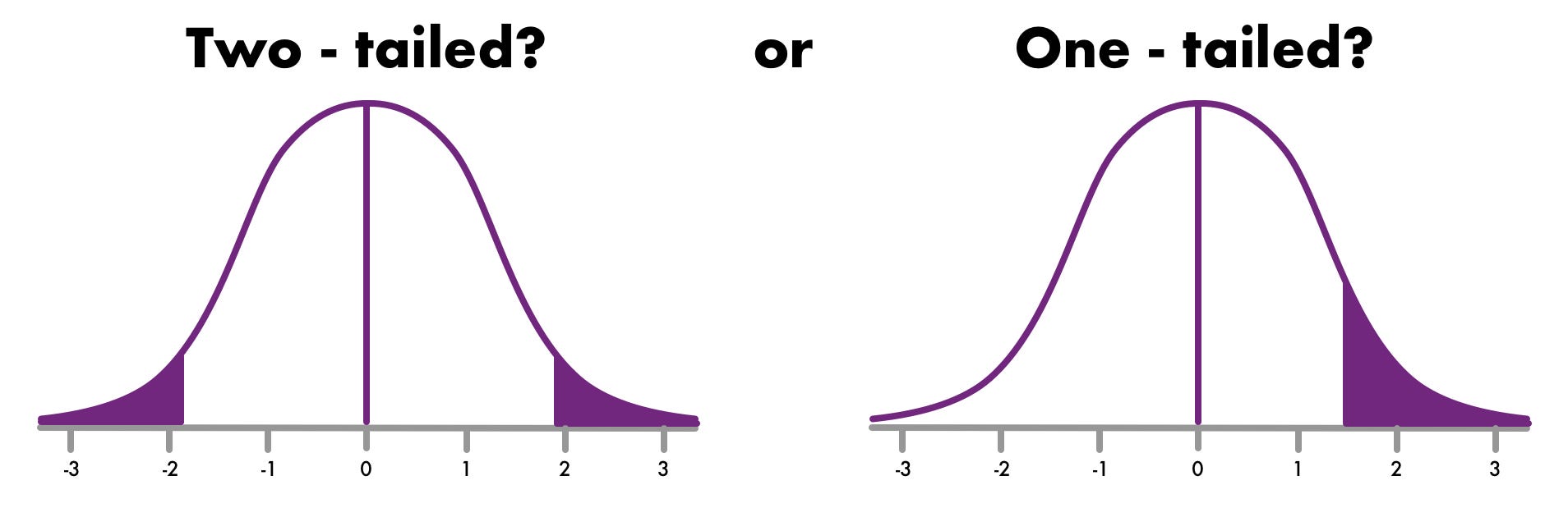
Image from https://towardsdatascience.com/hypothesis-testing-z-scores-337fb06e26ab
Directional tests are one-tailed (evaluate only one tail of the distribution) because they are investigating a specific direction of effect for the IV (e.g. increasing) while nondirectional tests are two-tailed (evaluate both tails of the distribution) because they are not specifying the direction of effect for IV.
Experimental and Control Groups
Basic scientific methodology requires an experimental and a control group. The experimental group receives the IV while the control group does not. If a difference between the groups can be detected then that difference may be attributable to the IV. If there is no difference between the groups the IV does not have an effect.
Another way to state this is that the null hypothesis assumes that there is no difference between the control and experimental groups (the groups or equal), while the alternative hypothesis assumes that there will be a difference between the groups.
Null hypothesis - experimental group = control group
Alternative Hypothesis - experimental group \(\neq\) control group
The null hypothesis is tested to answer the question, “Are these results due to chance?” Different statistical tests use different probability distributions to analyze the results of an experiment. The probability distributions allow us to see what is the probability associated with the results we obtained in our experiment.
Alpha
The probability that is shown through the probability distribution is compared to alpha. Alpha is an accepted scientific standard for determining the likelihood of rejecting the null hypothesis. Alpha is equal to .05 or 5%. So the standard that is accepted by the scientific community is that there is only a 5% chance or less that the findings in the experiment conducted are the result of chance alone. \[ \alpha = .05 \] The probability associated with the outcome of our experiment based on a probability distribution is known as the p value (p standing for probability)
Basic Statistical Formula
A really easy way to understand how most statistical outputs are generated is to understand this simple formula. \[ \frac{signal}{noise} \] Signal refers to what is known as systematic variation or variation that is introduced by an experiment. In the gasoline example, the additive that is supposed to increase gas mileage is systematic variation. The gasoline is being manipulated to try to increase gas mileage through the use of the additive. The more increase in gas mileage associated with the additive, the stronger the signal and the more likely the independent variable (in this case the additive) has a real effect.
Noise is like background noise or variation that exists, but wasn’t introduced through the experimental manipulation. This is often referred to as unsystematic variation. This is variation that exists for a variety of reasons. Going back to our gasoline mileage example, unsystematic variation could be differences in the cars used, differences in the road conditions or differences in the weather. Experimentors try to minimize this type of variation as much as possible, but there is always a certain amount of unsystematic variation
Measurement Error
One potential form of unsystematic variation is measurement error. For example, imagine that you weigh yourself every day for a whole week. Most likely there will be fluctuations in your weight during the week. It will be slightly higher one day and slightly lower another day with an average or mean that stays more consistent. Measurement error exists in any variable that we are attempting to measure. It is unavoidable to a certain extent because whatever we are attempting to measure, there will be certain fluctuations in the precision of measurement. Going back to our original formula, measurement error is our estimation of noise and although experiments are always trying to minimize error a certain amount will always be present. So another way to understand our primary formula is \[ statistics = \frac{experimental\;manipulation}{measurement\;error} \]
Confidence Intervals
One statistic to help analyze measurement error is called a confidence interval. A confidence interval is an interval of numbers between which we are 95% confident that the population mean is contained when drawn from a sample. According to Morling (2021) a confidence interval is composed of 3 components.
- Variability component - this is most often the standard deviation sd (remember that the sd if one of our basic measures of dispersion or variability)
- Sample size component - Usually this will be a calculation involving the number in the sample, most often symbolized by n.
- Constant associated with 95% - Here we’ll use the z score associated with 95 percent
Here is the basic formula for a confidence interval using z scores.
lower boundary of CI - \(\bar X - 1.96\) x \(\frac{s}{\sqrt{n}}\)
upper boundary of CI - \(\bar X + 1.96\) x \(\frac{s}{\sqrt{n}}\)
\(\frac{s}{\sqrt{n}}\) is known as the standard error of the mean and is the standard deviation divided by the square root of the number in the sample. 1.96 is the z score associated with the 95% percentile, thus, the 95% confidence interval.
Confidence Interval Example
Let’s imagine we have a sample of persons aged 40 to 50 who were trying to run on a treadmill at it’s fastest speed. This is a sample of times in seconds they were able to maintain a sprint at the treadmill’s fastest speed.
Then we can find the mean and standard deviation for this group of scores
sprint_mean <- mean(sprint)
sprint_sd <- sd(sprint)
Then we can use these scores to find the 95% confidence interval
lower <- sprint_mean - 1.96*sprint_sd/sqrt(21)
upper <- sprint_mean + 1.96*sprint_sd/sqrt(21)
lower
[1] 27.23457upper[1] 37.14638Based on this sample, we are 95% confident that the mean time for the population of 40 to 50-year-olds to sprint on the treadmill at its top speed is between 27.23 and 37.15 seconds.